Logistic regression is used for binary classification problems, where the goal is to predict the probability of an instance belonging to a particular class (0 or 1).

Here are some examples of application for logistic regression

1. Email Spam Detection
2. Political Prediction
3. Medical Diagnosis
4. Credit Scoring

Logistic regression can be used for both Binary Classification and Multi-class classification(Multinomial)

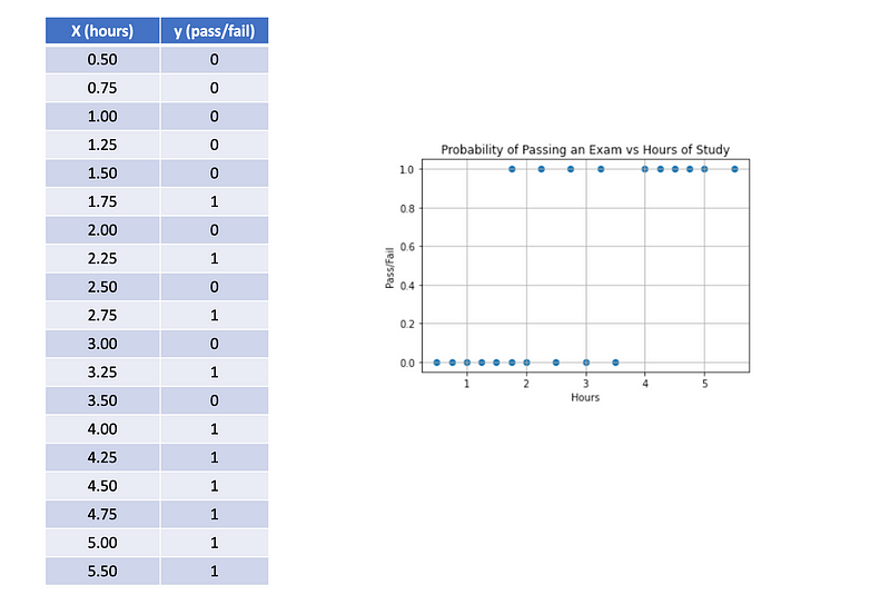
Consider the following example where we have data points indicating the number of hours each student spent studying and whether they passed (1) or failed (0).

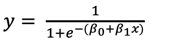
Model:

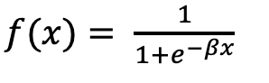
In logistic regression, the sigmoid function is employed to transform real values into a range of 0 to 1. This function guarantees that the model’s output can be interpreted as probabilities.

To implement this, we can utilize the sklearn module to fit the data. After fitting the model, we can obtain the coefficients and intercepts. The output looks like the following:

import numpy as np
import pandas as pd
from sklearn.linear_model import LogisticRegression
df = pd.DataFrame(
    {
        "hours": [0.50,0.75,1.00,1.25,1.50,1.75,1.75,2.00,2.25,2.50,2.75,3.00,3.25,3.50,4.00,4.25,4.50,4.75,5.00,5.50],
        "pass": [0, 0, 0, 0, 0, 0, 1, 0, 1, 0, 1, 0, 1, 0, 1, 1, 1, 1, 1, 1],
    }
)
model = LogisticRegression()
model.fit(df[['hours']],df['pass'])

print('Coefficients: ',np.round(model.coef_,3))
print('Intercept: ',np.round(model.intercept_,3))

Output:

Coefficients(beta 1) : [[1.149]] Intercept(beta 0): [-3.14]

Coefficient :

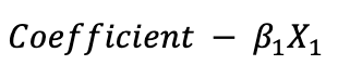
Ist is denotes as beta, represent the weights assigned to each input feature in the logistic regression model

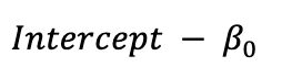
Intercept:

The intercept represents the log-odds of the positive class when all the input features are zero. In other words, it is the baseline log-odds before considering the effects of the features

Predict

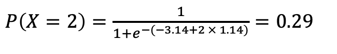
Given the values for beta 0 and beta 1, let’s predict the probability of a student who studies for 2 hours and estimate the likelihood of passing the exam.

Similarly, for a student studying 4 hours, let’s determine the estimated probability of passing the exam.

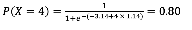
Let’s perform these calculations using our Python code to verify.

## Predict the probability of passing an exam for 2 hours and 4 hours
y_pred = model.predict_proba(np.array([2,4]).reshape(-1,1))
print(y_pred)

[0.30104715 0.81075008]

We obtained an approximate value from python code.

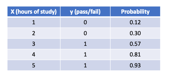
Now, to evaluate our model, the table below displays the estimated probabilities of passing the exam for 1,2,3,4 and 5 hours of study.

## Prediction and probability of passing an exam for 1,2,3,4 and 5 hours of study
y_pred = model.predict(np.array([1,2,3,4,5]).reshape(-1,1))
print("Pass/Fail Prediction", y_pred)
print("Probabilities", model.predict_proba(np.array([1,2,3,4,5]).reshape(-1,1))[:,1])

Pass/Fail Prediction [0 0 1 1 1]

Probabilities [0.12015954 0.30104715 0.57597882 0.81075008 0.93108619]

Plotting

Visualize the data points on a graph and observe the resulting curve.

import numpy as np
import matplotlib.pyplot as plt
# Define the logistic regression sigmoid function
def sigmoid(x, b0, b1):
    return 1 / (1 + np.exp(-(b0 + b1 * x)))

# Generate x values
x_values = np.linspace(0, 5, 100)

# Set your coefficients
b0 = -3.14 # replace with your actual intercept
b1 = 1.14  # replace with your actual coefficient

# Calculate corresponding sigmoid values
sigmoid_values = sigmoid(x_values, b0, b1)

# Create a scatter plot (your existing data)
plt.scatter(df['hours'], df['pass'], label='Scatter Plot')

# Plot the logistic regression sigmoid curve
plt.plot(x_values, sigmoid_values, label='Logistic Regression Sigmoid Curve', color='red')

# Customize the plot as needed
plt.title('Probability of Passing an Exam vs Hours of Study (Logistic Regression Sigmoid Curve)')
plt.xlabel('Hours of Study')
plt.ylabel('Probability of Passing an Exam')

# Show the plot
plt.show()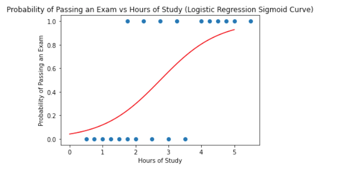

Model Evaluation

Model evaluation is crucial for assessing the performance of machine learning algorithms. In Python, the sklearn library provides a convenient tool for evaluating accuracy. By comparing predicted labels to actual ones, the accuracy_score function quantifies the model's correctness. This metric, expressed as a percentage, indicates the proportion of correct predictions among all predictions made.

## Model Evaluation
from sklearn.metrics import accuracy_score
y_pred = model.predict(df[['hours']])
print("Accuracy:",accuracy_score(df['pass'],y_pred))

Accuracy: 0.8

Correlation Matrix

The correlation matrix is a powerful tool in data analysis, revealing relationships between variables.It helps to visually depicted as a matrix, each cell represents the correlation between actual vs predicted as show below

## draw the correlation matrix
import seaborn as sns
sns.heatmap(confusion_matrix(df['pass'],y_pred),annot=True)
# add labels
plt.xlabel('Predicted')
plt.ylabel('Actual')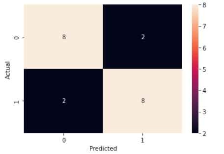

Cross Entropy Loss

## cross entropy loss for the above data
import numpy as np
import pandas as pd
from sklearn.metrics import log_loss
cross_entropy = log_loss(df['pass'],model.predict_proba(df[['hours']])[:,1])
print(f"Cross-Entropy (Log Loss): {cross_entropy:.4f}")

Cross-Entropy (Log Loss): 0.4109

A log loss of 0.4 is a metric indicating the average negative log-likelihood of the true labels given the predicted probabilities. Generally, lower log loss values are desirable, as they indicate better model performance. A log loss of 0.4 suggests that, on average, the predicted probabilities are reasonably close to the true labels.

However, the interpretation of log loss depends on the specific context of your problem and the distribution of your data. It’s often helpful to compare the log loss of your model to a baseline model or other models you might be considering for the task.

Here are some general guidelines for interpreting log loss:

• Log Loss of 0: Perfect predictions.
• Log Loss close to 0: Excellent model performance.
• Log Loss close to 0.5: Model is making random predictions.
• Log Loss above 0.5: Model performance may need improvement.
• Log Loss approaching infinity: Model is making very confident but incorrect predictions.

It’s essential to consider the characteristics of your specific dataset and the context of your problem when interpreting log loss values. Additionally, if log loss alone doesn’t provide sufficient insight into model performance, you may want to consider other metrics, such as accuracy, precision, recall, or F1 score, depending on the nature of your classification problem.

In the next chapter, we will explore the implementation of logistic regression for multinomial data.