In this blog post, we delve into the fascinating world of multiclass classification using logistic regression, specifically focusing on the recognition of handwritten digits.
import matplotlib.pyplot as plt
import pandas as pd
from sklearn.datasets import load_digits
digits = load_digits()
df = pd.DataFrame(digits.data)
df['target'] = digits.target
Understanding the Dataset:
Our dataset consists of 1,797 grayscale images, each representing a handwritten digit. The images are stored in a matrix, and by examining the shape of our dataframe, we find that it is (1797, 65), indicating 1,797 records with 65 columns.
Let's take a visual tour of our dataset by printing a sample of the handwritten digits.

import matplotlib.pyplot as plt
plt.gray()
for i in range(5):
    plt.subplot(1, 5, i + 1)
    plt.imshow(digits.images[i], cmap='gray')
    plt.title(f"Label: {digits.target[i]}")
    plt.axis('off')

handwritten image data of numbers
Dataset Splitting:
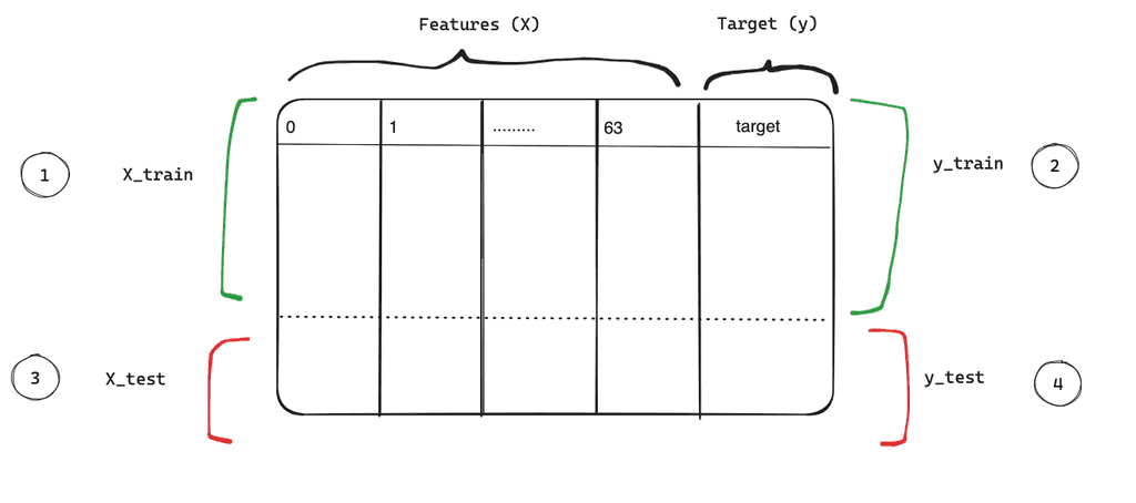
To effectively train and evaluate our logistic regression model, we need to split our dataset into training and testing sets. The features (X) are the grayscale image vectors, and the targets (y) represent the numbers from 0 to 9.

print(df['target'][0:5])
Keep the features and target in X and y variables
# Separate features (X) and target (y)
X = df.drop('target', axis='columns')
y = df['target']
print(X.shape)
print(y.shape)(1797, 64)
(1797,)from sklearn.model_selection import train_test_splitX_train, X_test, y_train, y_test = train_test_split(X,y,train_size=0.8, test_size=0.2)
print(X_train.shape)
print(X_test.shape)The resulting split yields a training set with 80% of the data (1,437 records) and a test set with the remaining 20% (360 records). The shape of the training set is (1437, 64), indicating 1,437 records with 64 features each, while the testing set has a shape of (360, 64).
Training
With our dataset split into training and testing sets, we are ready to start the training. Leveraging the power of scikit-learn, we'll employ a pipeline that includes feature scaling and logistic regression.
from sklearn.linear_model import LogisticRegression
from sklearn.pipeline import make_pipeline
from sklearn.preprocessing import StandardScaler

model = make_pipeline(StandardScaler(), LogisticRegression(max_iter=1000))

model.fit(X_train, y_train)
Our model is now equipped to recognize patterns within the grayscale images of handwritten digits. The use of a pipeline ensures that our features are appropriately scaled before being fed into the logistic regression algorithm.
To assess the performance of our trained model, we turn to a key metric: accuracy. The model's accuracy can be obtained using the model.score method.
model.score(X_test, y_test)0.9638888888888889
This gives us an initial glimpse into how well our model performs on the testing set.
Model evaluation
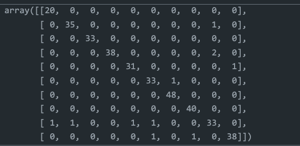
The confusion matrix provides a detailed breakdown of correct and incorrect predictions for each class (digit).
from sklearn.metrics import confusion_matrix
y_predicted = model.predict(X_test)
cm = confusion_matrix(y_test, y_predicted)
cm
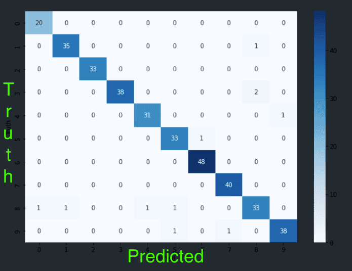
The confusion matrix heatmap provides a visual representation of our model's performance for each digit. For instance:
from seaborn import heatmap
plt.figure(figsize=(10,7))
heatmap(cm, annot=True, fmt='d', cmap='Blues')
plt.xlabel('Predicted')
plt.ylabel('Truth')
- For digit 0, our model correctly predicted 20 instances and failed once.
- For digit 1, the model made 35 correct predictions and one incorrect prediction.
This visual representation allows us to identify areas where our model excels and where it may need improvement, providing valuable insights for further refinement.
Conclusion
In this blog post, we've laid the foundation for our exploration of multiclass classification using logistic regression. By preparing our dataset of handwritten digits, splitting it into training and testing sets, and understanding the structure of our features and targets. In the next blog post we will dive into how to apply classification to ordinal dataset.
